Debunking the Audio Myth: Why Class D Amplifiers Are Fully Analog (And Not Digital)

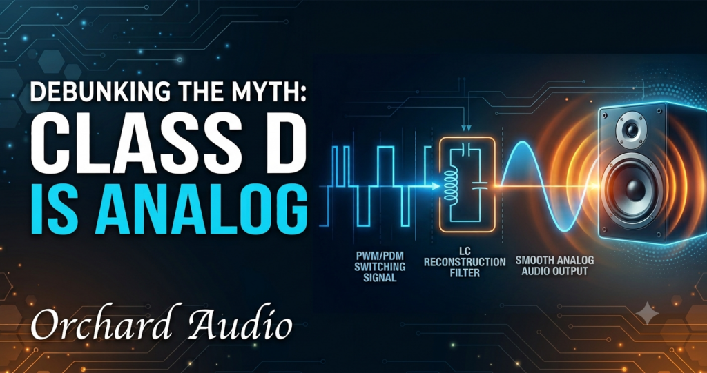
Mention the term “Class D” to a room of audio enthusiasts, and the vast majority will tell you that the “D” stands for “digital.” It is one of the most deeply ingrained misconceptions in high-end audio, driven by a simple visual intuition: because a Class D output stage rapidly switches between two fixed voltage states—producing what appears to be a binary, two-level square wave—it must be digitizing the musical signal.

For decades, this myth led purists to assume that Class D amplifiers inherently chop up delicate analog music into discrete binary samples, introducing quantization steps, bit-depth limitations, and clock jitter. Some audiophiles even assume all Class D circuits operate identically using fixed-frequency Pulse Width Modulation (PWM).

Here is the rigorous engineering reality: Class D power amplifiers are 100% continuous analog systems. There is no digital-to-analog conversion, no sampling clock grid, no binary code, and zero quantization error anywhere inside a traditional Class D circuit. Furthermore, Class D is a broad engineering category that encompasses both Pulse Width Modulation (PWM) and Pulse Density Modulation (PDM) / self-oscillating feedback architectures.

The Naming Misconception: Where Did ‘Class D’ Come From?

To understand why Class D is fully analog, we must first clear up the taxonomy of audio amplifier classification. Amplifier classes are defined strictly by the conduction angle of the output transistors over a 360-degree input sine wave:

• Class A: The output transistor conducts current during the full 360 degrees of the input cycle. It offers high linearity but very low energy efficiency (typically 15–20%), dissipating the remaining electrical power as waste heat.

• Class B: Two transistors operate in push-pull; each conducts for 180 degrees (half the cycle). Efficiency improves to roughly 70%, but introduces severe crossover distortion at the zero-crossing point.

• Class AB: A hybrid design where both transistors remain biased ON for slightly more than 180 degrees, eliminating crossover distortion while preserving reasonable power efficiency.

• Class C: The transistor conducts for less than 180 degrees. Highly efficient, but generates heavy harmonic distortion, making it suitable for RF radio transmitters but unusable for high-fidelity audio.

When British engineer Alec Reeves and subsequent researchers developed a switching-mode topology in the mid-20th century, it was assigned the next available letter in the IEEE classification sequence: Class D.

The letter “D” has zero connection to the word “digital.” In fact, when Class D principles were first patented, commercial digital audio technology (such as CDs, PCM streams, or digital signal processors) did not exist.

Defining Analog vs. Digital: The Physics of Information Representation

To evaluate whether a circuit is analog or digital, we must look at how electrical signals represent information in time and amplitude domains.

Engineering Axis	Analog Domain	Digital Domain
Time Reference	Continuous in time (Infinite temporal resolution)	Discrete in time (Sampled at fixed clock intervals)
Amplitude Domain	Continuous real values bounded by voltage rails	Quantized discrete steps (e.g., 65,536 levels for 16-bit)
Signal Representation	Physical continuous variables (voltage, pulse width, frequency)	Numerical abstractions (Binary code: 0s and 1s)
Error Mechanics	Continuous thermal noise floor & phase shift	Quantization noise, bit rounding, & clock jitter

 

An analog system is continuous in both time and amplitude. Every physical parameter—whether it is the voltage on a wire, the position of a speaker cone, or the width of a pulse—can take on any real value within its operating range, changing smoothly without discrete jumps.

A digital system is discrete. It takes continuous physical variables and samples them at specific clock ticks, rounding the values to the nearest entry on a mathematical quantization ladder. A digital signal consists of abstract mathematical numbers, not direct physical representations.

The Core Physics: Why a Square Wave / Pulse Signal is Fully Analog

The central point of visual confusion in Class D amplifiers is the switching waveform itself. When viewed on an oscilloscope, the signal flips rapidly between two voltage levels, resembling a clean square wave or pulse train. Because digital logic circuits also use two-state levels (high/low), it is tempting to conclude that a square wave is digital.

However, in electrical physics, a physical square wave or pulse train is entirely analog.

Continuous Time Resolution of Switching Edges

In a digital circuit, signal transitions are synchronized to a master clock. A bit can only change state on a specific clock edge tick.

In an analog Class D amplifier, the switching transitions (the leading and trailing edges of the pulse) are not locked to a clock grid. The exact moment an edge occurs can shift continuously by fractions of a picosecond in direct response to the continuous analog input voltage. Because the pulse duration (width) or pulse repetition density can take on an infinite number of real values, the time domain resolution of the signal is infinite and continuous.

Physical Parameters Bounded by Real Circuit Physics

A theoretical digital square wave represents abstract numbers (0 and 1). A physical square wave traveling through a circuit is a real analog AC voltage wave governed by Maxwell’s equations and Fourier analysis.

According to Fourier analysis, a physical square wave is composed of an infinite sum of continuous analog sinusoidal harmonics:

Or in simpler terms, a square wave is the sum of a sine wave and all of its odd harmonics. Here is a visual representation of how sine waves can sum to become square waves;

When a switching amplifier generates a pulse waveform, it is sending real continuous power through a circuit. The pulse contains physical parameters—slew rates, rise times, fall times, ringing, and continuous voltage variations—that are shaped by physical inductors, capacitors, and transistor gate characteristics, not software code.

Information Encoded in Time Rather Than Amplitude

In a traditional Class A or AB amplifier, audio information is encoded in continuous voltage amplitude. In a Class D amplifier, information is translated into continuous time duration (pulse width or pulse density). Moving information from the amplitude domain to the time domain does not make it digital; it remains continuous analog encoding.

Frequency modulation (FM) does something structurally similar — amplitude information becomes a continuously variable instantaneous frequency — and nobody argues FM radio is a digital transmission format.

Class D Topologies: Pulse Width Modulation (PWM) vs. Pulse Density Modulation (PDM)

Class D amplifiers are not all built the same. Lumping all switching amplifiers into a single “PWM” bucket ignores key architectural developments in modern high-fidelity audio.

Pulse Width Modulation (PWM) — Fixed Carrier Frequency

In standard PWM amplifiers, an incoming analog audio signal is compared against a fixed-frequency triangular or sawtooth reference oscillator (typically between 300 kHz and 500 kHz).

When the audio voltage exceeds the triangle wave voltage, the comparator output goes high; when it falls below, the output goes low. The carrier frequency remains constant, while the width (duty cycle) of each pulse varies proportionally with the analog input level.

Pulse Density Modulation (PDM) & Self-Oscillating Loops

Rather than relying on a fixed internal oscillator, advanced audiophile Class D designs—such as those implemented in Orchard Audio’s Starkrimson architectures—utilize Pulse Density Modulation (PDM) within self-oscillating control loops.

In a self-oscillating PDM architecture:

• Dynamic Frequency Modulation: The circuit uses a continuous analog feedback loop that oscillates naturally. The switching frequency adjusts dynamically in real time depending on the input signal dynamics.

• Variable Pulse Density: Information is encoded by changing both the repetition density and duration of the switching pulses, optimizing instantaneous transient response.

• Elimination of Clock Noise: Without a fixed carrier oscillator, there is no fixed clock spike in the RF spectrum, reducing intermodulation artifacts and improving control loop stability across varying speaker loads.

 

The Light Switch Analogy: Understanding Switching Efficiency

A simple physical comparison helps illustrate why switching delivers efficiency without altering signal continuity:

• Linear Dimmer (Class A/AB): Like an adjustable resistor in a lighting circuit. To dim a room to 50% brightness, the linear switch absorbs 50% of the electrical energy, dissipating it as heat behind the wall plate.

• Switching Control (Class D): Like flipping a light switch ON and OFF 1,000,000 times per second. By leaving the switch ON for 50% of each cycle and OFF for 50%, human visual persistence perceives 50% brightness—and the switch itself remains completely cool.

In audio, speaker drivers act like the human eye: they cannot respond to megahertz-level switching pulses, so they naturally integrate the high-speed energy stream into continuous mechanical motion.

From Early Silicon to Gallium Nitride (GaN): How Switching Transistors Evolved

If Class D is purely analog, why did early Class D amplifiers in the 1990s earn a reputation for sounding harsh or “dry”?

The issue was not the analog switching concept, but the physical limitations of legacy Silicon MOSFET transistors. Early silicon devices were slow, switching at lower frequencies (100–300 kHz). This required heavy output filters near the audible band, causing high-frequency phase shifts and non-linear “dead time***” crossover distortion.

The advent of Gallium Nitride (GaN) FETs transformed switching performance:

• Ultra-Fast Switching Rates: GaN devices switch up to 10 times faster than silicon MOSFETs, pushing switching frequencies above 1.0 MHz (1,000,000 Hz). Our Starkrimson 25 Mono Premium amplifers switch at 1.1MHz.

• Near-Zero Dead Time: GaN switches toggle almost instantaneously, virtually eliminating dead-time crossover distortion.

• Transparent Filtering: Switching above 1 MHz allows lightweight output filters with flat frequency response and zero audible phase shift across complex speaker impedances.

*** Dead time is the brief interval in a Class‑D amplifier’s switching cycle during which both power devices (MOSFETs or GaN FETs) are intentionally turned off. This pause prevents shoot‑through—where both devices conduct simultaneously and short the supply rails. During dead time, the output node is not actively driven, so the speaker load is momentarily left to “coast” based on its own current. This uncontrolled interval introduces distortion because the amplifier cannot precisely shape the output waveform. Research shows that dead time is a dominant contributor to nonlinearity and harmonic distortion in Class‑D output stages. To compensate for this loss of control, more feedback is required—especially as dead time increases. Minimizing dead time is therefore critical for high‑fidelity Class‑D performance.

Orchard Audio’s amplifiers use extremely small dead times of < 5 nanoseconds (a billionth of a second), which is far below typical industry values and helps maintain exceptionally low distortion without a lot of feedback.

PWM vs. PDM vs. True Digital PCM: Technical Comparison

Parameter	Digital PCM Audio	Class D PWM	Class D PDM (Self-Oscillating)
Signal Representation	Discrete Binary Numbers (0/1)	Continuous Time Waveform	Continuous Time Waveform
Time Reference	Fixed Master Clock Grid	Fixed Carrier Oscillator	No Clock (Self-Oscillating Loop)
Amplitude Encoding	Quantized Binary Bits	Continuous Pulse Width	Continuous Pulse Density
Signal Domain	Digital Domain	100% Analog Domain	100% Analog Domain

 

Where The “Digital” Label Does Apply

There is a real, separate category of “digital-input” Class-D amplifiers, where a PCM or DSD/PDM bitstream feeds a digital PWM modulator (implemented in a DSP, FPGA, or dedicated logic) before ever reaching the switches. In those designs, everything up to the gate driver genuinely is digital: discrete-time, discrete-amplitude, clock-governed. But that’s a design choice about the input and control stage, not a property of Class D as a topology. The classic and still very common alternative — self-oscillating or comparator-based, “naturally sampled” Class D — has no ADC, no digital clock domain, and no quantization anywhere between the analog input and the loudspeaker terminals.

 

Frequently Asked Questions (FAQ)

Q1: Does playing a vinyl record through a Class D amplifier convert it to digital?

No. The continuous voltage signal from your phono cartridge passes through the amplifier entirely in the continuous analog domain. It is never sampled, digitized, or converted into binary code.

Q2: Why do some products claim to be “Full Digital Amplifiers”?

There are specialized devices called Power DACs or Equibit amplifiers that accept PCM digital inputs and convert them directly to PWM. However, standard Class D power amplifiers accept analog voltage inputs and operate entirely as analog circuits.

Q3: Is a square wave created by digital software the same as a physical switching square wave?

No. A digital square wave in software is an array of mathematical values. A physical square wave in an amplifier is a continuous electrical waveform governed by continuous rise times, spectral harmonics, and analog circuit interactions.

Explore Modern GaN Class D Amplification

Class D is not digital—it is an advanced, highly efficient form of continuous analog power amplification. By combining Gallium Nitride (GaN) switching devices with self-oscillating Pulse Density Modulation (PDM) control loops, modern amplifiers deliver unprecedented clarity, bandwidth, and control.

To explore how GaN technology and self-oscillating PDM architectures are implemented in state-of-the-art audiophile components:

• Product Catalog: Explore Orchard Audio’s Starkrimson GaN monoblock, stereo, and amplifer modules at www.orchardaudio.com/shop.

• Engineering Support: Connect directly with lead designer Leo Ayzenshtat regarding custom audio systems and engineering inquiries at www.orchardaudio.com/contact-us.

 

References & Academic Literature

1. Groenenberg, R., Putzeys, B., van der Hulst, P., & Veltman, A. (2006). All Amplifiers Are Analogue, But Some Amplifiers Are More Analogue Than Others. AES Convention Paper 6690, 120th AES Convention, Paris. https://aes2.org/publications/elibrary-page/?id=13494
2. Putzeys, B. (2003). Digital Audio’s Final Frontier. IEEE Spectrum, 40(4). https://spectrum.ieee.org/digital-audios-final-frontier
3. Wikipedia Contributors. Class-D amplifier. Wikipedia, The Free Encyclopedia. https://en.wikipedia.org/wiki/Class-D_amplifier
4. ECE Department, UC Riverside. The Class-D Amplifier. EE135 Course Notes, Department of Electrical & Computer Engineering, University of California, Riverside. https://intra.ece.ucr.edu/~rlake/EE135/Class_D_amp_notes_AL.pdf
5. Electronic Design. Digital Versus Analog Power Control — A Fight To The… Draw? Electronic Design. https://www.electronicdesign.com/technologies/embedded/article/21767846/digital-versus-analog-power-controla-fight-to-the-draw
6. Extron Electronics. Class D Amplifiers — Not “Just Audio.” Extron Technical Articles. https://www.extron.com/article/ts122001
7. Texas Instruments: A Comprehensive Study of Class D Amplifier Technology. https://e2e.ti.com/cfs-file/__key/communityserver-discussions-components-files/6/A-comprehensive-study-of-class-D-amplifier-technology.pdf